How to Find the General Solution of an Augmented Matrix
Solving a linear system with matrices using Gaussian elimination
After a few lessons in which we have repeatedly mentioned that we are covering the basics needed to later learn how to solve systems of linear equations, the time has come for our lesson to focus on the full methodology to follow in order to find the solutions for such systems.
What is Gaussian elimination
Gaussian elimination is the name of the method we use to perform the three types of matrix row operations on an augmented matrix coming from a linear system of equations in order to find the solutions for such system. This technique is also called row reduction and it consists of two stages: Forward elimination and back substitution.
These two Gaussian elimination method steps are differentiated not by the operations you can use through them, but by the result they produce. The forward elimination step refers to the row reduction needed to simplify the matrix in question into its echelon form. Such stage has the purpose to demonstrate if the system of equations portrayed in the matrix have a unique possible solution, infinitely many solutions or just no solution at all. If found that the system has no solution, then there is no reason to continue row reducing the matrix through the next stage.
If is possible to obtain solutions for the variables involved in the linear system, then the Gaussian elimination with back substitution stage is carried through. This last step will produce a reduced echelon form of the matrix which in turn provides the general solution to the system of linear equations.
The Gaussian elimination rules are the same as the rules for the three elementary row operations, in other words, you can algebraically operate on the rows of a matrix in the next three ways (or combination of):
- Interchanging two rows
- Multiplying a row by a constant (any constant which is not zero)
- Adding a row to another row
And so, solving a linear system with matrices using Gaussian elimination happens to be a structured, organized and quite efficient method.
How to do Gaussian elimination
The is really not an established set of Gaussian elimination steps to follow in order to solve a system of linear equations, is all about the matrix you have in your hands and the necessary row operations to simplify it. For that, let us work on our first Gaussian elimination example so you can start looking into the whole process and the intuition that is needed when working through them:
Example 1
Notice that at this point, we can observe that this system of linear equations is solvable with a unique solution for each of its variables. What we have performed so far is the first stage of row reduction: Forward elimination. We can continue simplifying this matrix even more (which would take us to the second stage of back substitution) but we really don't need to since at this point the system is easily solvable. Thus, we look at the resulting system to solve it directly:
From this set, we can automatically observe that the value of the variable z is: z=-2. We use this knowledge to substitute it on the second equations to solve for y, and the substitute both y and z values on the first equations to solve for x:
More Gaussian elimination problems have been added to this lesson in its last section. Make sure to work through them in order to practice.
Difference between gaussian elimination and gauss jordan elimination
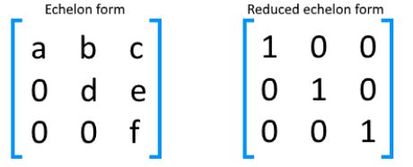
The difference between Gaussian elimination and the Gaussian Jordan elimination is that one produces a matrix in row echelon form while the other produces a matrix in row reduced echelon form. A row echelon form matrix has an upper triangular composition where any zero rows are at the bottom and leading terms are all to the right of the leading term from the row above. Reduced echelon form goes beyond by simplifying much more (sometimes even reaching the shape of an identity matrix).
The history of Gaussian elimination and its names is quite interesting, you will be surprised to know that the name "Gaussian" was attributed to this methodology by mistake in the last century. In reality the algorithm to simultaneously solve a system of linear equations using matrices and row reduction has been found to be written in some form in ancient Chinese texts that date to even before our era. Then in the late 1600's Isaac Newton put together a lesson on it to fill up something he considered as a void in algebra books. After the name "Gaussian" had been already established in the 1950's, the Gaussian-Jordan term was adopted when geodesist W. Jordan improved the technique so he could use such calculations to process his observed land surveying data. If you would like to continue reading about the fascinating history about the mathematicians of Gaussian elimination do not hesitate to click on the link and read.
There is really no physical difference between Gaussian elimination and Gauss Jordan elimination, both processes follow the exact same type of row operations and combinations of them, their difference resides on the results they produce. Many mathematicians and teachers around the world will refer to Gaussian elimination vs Gauss Jordan elimination as the methods to produce an echelon form matrix vs a method to produce a reduced echelon form matrix, but in reality, they are talking about the two stages of row reduction we explained on the very first section of this lesson (forward elimination and back substitution), and so, you just apply row operations until you have simplified the matrix in question. If you arrive to the echelon form you can usually solve a system of linear equations with it (up until here, this is what would be called Gaussian elimination). If you need to continue the simplification of such matrix in order to obtain directly the general solution for the system of equations you are working on, for this case you just continue to row-operate on the matrix until you have simplified it to reduced echelon form (this would be what we call the Gauss-Jordan part and which could be considered also as pivoting Gaussian elimination).
We will leave the extensive explanation on row reduction and echelon forms for the next lesson, for now you need to know that, unless you have an identity matrix on the left hand side of the augmented matrix you are solving (in which case you don't need to do anything to solve the system of equations related to the matrix), the Gaussian elimination method (regular row reduction) will always be used to solve a linear system of equations which has been transcribed as a matrix.
Gaussian elimination examples
As our last section, let us work through some more exercises on Gaussian elimination (row reduction) so you can acquire more practice on this methodology. Throughout many future lessons in this course for Linear Algebra, you will find that row reduction is one of the most important tools there are when working with matrix equations. Therefore, make sure you understand all of the steps involved in the solution for the next problems.
Example 2
Example 3
For this system we know we will obtain an augmented matrix with three rows (since the system contains three equations) and three columns to the left of the vertical line (since there are three different variables). On this case we will go directly into the row reduction, and so, the first matrix you will see on this process is the one you obtain by transcribing the system of linear equations into an augmented matrix.
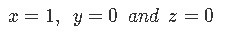
Notice how we can tell right away that the variable z is equal to zero for this system since the third row of the resulting matrix shows the equation -9z = 0. We use that knowledge and check the second row of the matrix which would provide the equation 2y - 6z = 0, plugging the value of z = 0 into that equation results in y also being zero. Thus, we finally substitute both values of y and z into the equation that results from the first row of the matrix: x + 4y + 3z = 1, since both y and z are zero, then this gives us x = 1. And so, the final solution to this system of equations looks as follows:
-
Equation 16: Final solution to the system of equations
Example 4
From which we can see that the last row provides the equation: 6z = 3 and therefore z = 1/2. We substitute this in the equations resulting from the second and first row (in that order) to calculate the values of the variables x and y:
Example 5
Example 6
To finalize our lesson for today we have a link recommendation to complement your studies: Gaussian elimination an article which contains some extra information about row reduction, including an introduction to the topic and some more examples. As we mentioned before, be ready to keep on using row reduction for almost the whole rest of this course in Linear Algebra, so, we see you in the next lesson!
How to Find the General Solution of an Augmented Matrix
Source: https://www.studypug.com/algebra-help/solving-a-linear-system-with-matrices-using-gaussian-elimination